calculating PI

Programming exercise

In contrast to the simple method described below, the first exercise should calculates our own PI.

pi

[1] 3.141593

The following is a step-by-step guide to putting the first programming skills from the lesson into practice.

Basic idea

As Ven showed in the first lesson…

… if we throw thousands of random placed darts into a square field, the number of darts that fall into the enclosed circle should represent the area of that circle in relation to the area of the square.

In the following we will try to confirm this with our own programming skills.

1. Step

Generation of a random position for a single dart within a square. The square extends from -1 to +1 in the X-direction, as well as in the Y-direction.
Use a random number generator for a uniform distribution and save the result in the two variables x and y (GAP are placeholder)

x <- runif(n = GAP, min = GAP, max = GAP)
y <- GAP

Feasible solution

x <- runif(n = 1, min = -1, max = 1)
y <- runif(n = 1, min = -1, max = 1)

2. Step

Now calculate the distance from this position to the center. You can use the following simplified formula for our chosen square

dist <- x**2 + y**2
print(dist)

[1] 0.780845

3. Step

Create a decision rule and print “inside” if the point is inside the circle or “outside” if it is not.

if (dist <= GAP) {
  GAP
} else {
  GAP
}

Feasible solution

if (dist <= 1) {
  print("inside")
} else {
  print("outside")
}

[1] "inside"

4. Step

Create now a loop (use for or while statement) and execute the code from steps 1 to 3 within it. You should get something like that now

Hint: Use may 10 iteration for the beginning

Feasible solution

for (i in 1:10) {
  x <- runif(n = 1, min = -1, max = 1)
  y <- runif(n = 1, min = -1, max = 1)
  dist <- x**2 + y**2
  if (dist <= 1) {
    print("inside")
  } else {
    print("outside")
  }
}

[1] "inside"
[1] "inside"
[1] "inside"
[1] "outside"
[1] "inside"
[1] "outside"
[1] "inside"
[1] "inside"
[1] "inside"
[1] "inside"

5. Step

Copy now the code from Step 4 and modify it in a way that instead of outputting a result for each point, it sums up the number of “insides”.

Use something like that,

n_insides <- 0
n_insides <- n_insides + 1
print(n_insides)

[1] 1

or more elegant write the results in a vector.

v_insides <- rep(x = 0, 10)
v_insides[2] <- 1
print(v_insides)

 [1] 0 1 0 0 0 0 0 0 0 0

If you use 1000 iteration you should became such a number

[1] 780

Feasible solution

n <- 1000
v_insides <- rep(x = 0, n)
for (i in 1:n) {
  x <- runif(n = 1, min = -1, max = 1)
  y <- runif(n = 1, min = -1, max = 1)
  dist <- x**2 + y**2
  if (dist <= 1) {
    v_insides[i] <- 1
  }
}

Final Step

As the final step, you now need to calculate PI from your result and compare it with the real one ;-)

Feasible solution

selfmade_pi <- sum(v_insides) / length(v_insides) * 4
print(selfmade_pi)

[1] 3.096

if (selfmade_pi == pi) {
  print("YOU ARE UNBELIEFABLE")
} else {
  print("Try more iterations !!! (or try the function round)")
}

[1] "Try more iterations !!! (or try the function round)"

Outlook

If you, as we hoped, have been playing around with the code, you’ve probably noticed that it takes exponentially more time with a larger number of iterations! Therefore, here are some ways to optimize the code.

Loops and decision rules

These are very helpful because they are easy to read and interpret. However, they are very slow! Using the analogy Ven has used, each line is a page in a book. A loop means you constantly have to flip back and forth through the pages. In contrast, vector operations are much faster because it is already known in advance which operations need to be performed for the given values.

Here a first example

Although 10e8 iterations are performed here, it computes almost without any delay.

Hint: You may try to understand why this gives the same result.

n <- 1e8
data <- data.frame(
  x = runif(n = n, min = -1, max = 1),
  y = runif(n = n, min = -1, max = 1)
)
data$dist <- data$x * data$x + data$y * data$y
data$inside <- 2 - ceiling(data$dist)
selfmade_pi_opt1 <- sum(data$inside) / length(data$inside) * 4

head(data)

           x          y      dist inside
1 -0.6068475 -0.9722662 1.3135654      0
2 -0.5128652 -0.7091304 0.7658966      1
3  0.9976461 -0.8307470 1.6854383      0
4  0.5341546  0.5912639 0.6349140      1
5 -0.6608721  0.3332499 0.5478075      1
6 -0.6316362  0.9139095 1.2341949      0

As you can see, this way we already arrive a more precise solution much faster.

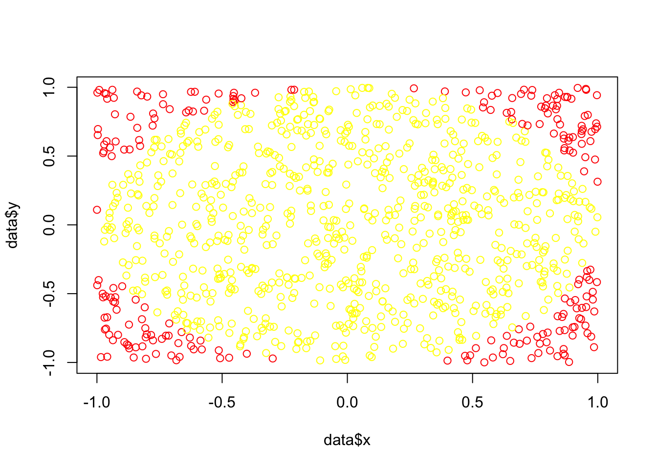
selfmade_pi

[1] 3.096

selfmade_pi_opt1

[1] 3.141585

pi

[1] 3.141593

Plot of Dart-positions

Other ways of optimization

R is a programming language for lazy people. Often, functions have preset default values, which in this example are even helpful. In others, it is very annoying because it makes the code harder to read. So you can love it or hate it, it’s up to you ;-)

Hint: May try ?runif to understand why this gives still the same result.

n <- 1e8
data <- data.frame(
  x = runif(n = n),
  y = runif(n = n)
)
data$dist <- data$x * data$x + data$y * data$y
data$inside <- 2 - ceiling(data$dist)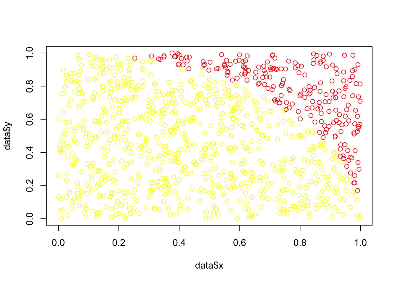
selfmade_pi_opt2 <- sum(data$inside) / length(data$inside) * 4

selfmade_pi

[1] 3.096

selfmade_pi_opt1

[1] 3.141585

selfmade_pi_opt2

[1] 3.14157

pi

[1] 3.141593

Hint: Plot of new Dart-positions

Explanation

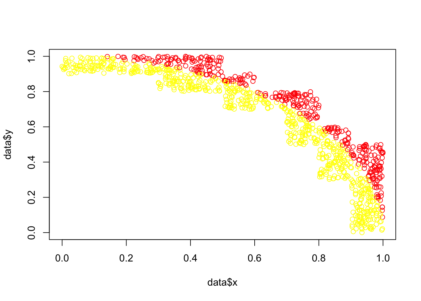
Since the effect of reducing the total area to a quarter is rather small, here is a clearer version. We now throw the darts only into fields where we expect a distinction. For fields in the 10x10 grid where we already know the answer, we do not throw any darts.

Feasible solution

n <- round(1e8 / 21, 0)
quader <- c(
  1,
  1,
  1,
  1,
  1,
  9 / 10,
  9 / 10,
  9 / 10,
  8 / 10,
  8 / 10,
  8 / 10,
  7 / 10,
  6 / 10,
  6 / 10,
  5 / 10,
  4 / 10,
  5 / 10,
  4 / 10,
  3 / 10,
  2 / 10,
  1 / 10
)
data <- data.frame(
  x = runif(n = n * length(quader), min = quader - 1 / 10, max = quader),
  y = runif(n = n * length(quader), min = rev(quader) - 1 / 10, max = rev(quader))
)
data$dist <- data$x * data$x + data$y * data$y
data$inside <- 2 - ceiling(data$dist)
selfmade_pi_opt3 <- (sum(data$inside) + n * 65) / (n * 100) * 4

selfmade_pi

[1] 3.096

selfmade_pi_opt1

[1] 3.141585

selfmade_pi_opt2

[1] 3.14157

selfmade_pi_opt3

[1] 3.141601

pi

[1] 3.141593